
ResInsight computes several derived results. In this section we will explain what they are, and briefly how they are calculated.
Derived Results for Eclipse Cases
ResInsight calculates several derived cell properties that is made available as Static or Dynamic cell properties. The derived results listed at the bottom of the Static result properties, are shown below.
Transmissibility Normalized by Area
The transmissibility for cells and Non-Neighbor Connections (NNCs) are dependent on both cell properties and geometry. ResInsight normalizes TRANX, TRANY and TRANZ with the overlapping flow area for both neighbor cells and NNC-cells. The results are named riTRANXbyArea, riTRANYbyArea and riTRANZbyArea respectively.
The normalized transmissibilities make it easier to compare and check the flow capacity visually. This can be useful when history matching pressure differences across a fault.
Overall Transmissibility Multiplier
Transmissibility can be set or adjusted with multiple keywords in an Eclipse data deck. To visualize the adjustments made, ResInsight calculates a multiplicator for the overall change. First unadjusted transmissibilities for all neighbor cells and NNCs are evaluated based on geometry and permeabilities, similar to the NEWTRAN algorithm in Eclipse. For x- and y-directions, the NTG parameter is also included. The results are named riTRANX, riTRANY and riTRANZ respectively.
The TRANX, TRANY and TRANZ used in the simulation are divided by the ResInsight calculated transmissibilities and the resulting multiplicators are named riMULTX, riMULTY and riMULTZ respectively. The derived properties are listed under Static properties. The riMULT-properties are useful for quality checking consistence in user input for fault seal along a fault plane.
Directional Combined Results
Cell properties with names ending in I, J, K, X, Y, or Z, and an optional “+” or “-“ are combined into derived results post-fixed with IJK, or XYZ depending on their origin. (Eg. the static cell properties MULTX, MULTY, MULTZ, and their negatives are combined into the result MULTXYZ, while the dynamic cell properties FLRGASI, FLRGASJ, FLRGASK are combined to FLRGASIJK).
These combined cell properties visualize the property as a color in all directions combined when selected in as a Cell Result and Separate Fault Result.
The face of a cell is then colored based on the value associated with that particular face. The Positive I-face of the cell gets the cell X/I-value, while the J-face gets the Y/J-value etc. The negative faces, however, get the value from the neighbor cell on that side. The negative I-face gets the X-value of the IJK-neighbor in negative I direction, and so on for the J- and K-faces.
The directional combined parameters available are:
- Static Properties
- TRANXYZ (inluding NNCs)
- MULTXYZ
- riTRANXYZ (inluding NNCs)
- riMULTXYZ (inluding NNCs)
- riTRANXYZbyArea (inluding NNCs)
- Dynamic Properties
- FLRWATIJK (inluding NNCs)
- FLROILIJK (inluding NNCs)
- FLRGASIJK (inluding NNCs)
- Generated
- Octave generated results with same name but ending with I,J and K will also be combined into a
<name>IJKcell property.
- Octave generated results with same name but ending with I,J and K will also be combined into a
Completion Type
The dynamic cell property named Completion Type is calculated from the intersections between Completions and the grid cells. All grid cells intersected by a completion will be assigned a color based on the type of completion that intersects the cell.
If a cell is completed with multiple completions, the following priority is used : Fracture, Fishbones, and Perforation Interval.
Identification of Questionable NNCs
In the process of normalizing transmissibility by the overlapping flow area, the NNCs in the model without any shared surface between two cells are identified. These NNCs are listed in the Faults/NNCs With No Common Area folder. These NNCs are questionable since flow normally is associated with a flow area.
Water Flooded PV
Water Flooded PV, also called Number of flooded porevolumes shows the amount of flow from a selected set of simulation tracers into a particular cell, compared to the cells mobile pore volume. A value of 1.0 will tell that the tracers accumulated flow into the cell has reached a volume equal to the mobile pore volume in the cell.
Derived Geomechanical results
ResInsight calculates several of the presented geomechanical results based on the native results present in the odb-files.
Relative Results (Time Lapse Results)
ResInsight can calculate and display relative results, sometimes also referred to as Time Lapse results. When enabled, every result variable is calculated as :
Value’(t) = Value(t) - Value(BaseTime)
Enable the Enable Relative Result option in the Relative Result Options group, and select the appropriate Base Time Step.
Each variable is then post-fixed with “_DTimeStepIndex” to distinguish them from the native variables.
Note: Relative Results calculated based on Gamma values are calculated slightly differently:
Gamma_Dn = ST_Dn / POR_Dn
Derived Result Fields
The calculated result fields are:
- Nodal
- COMPACTION (Magnitude of compression)
- Element Nodal and Integration Points
- ST (Total Stress)
- All tensor components
- Principals, with directions (Siinc, Siazi)
- STM (Mean total stress)
- Q (Deviatoric stress)
- Gamma (Stress path)
- SE (Effective Stress)
- All tensor components
- Principals, with directions
- SEM (Mean effective stress)
- SFI
- FOS
- DSM
- E (Strain)
- All tensor components
- EV (Volumetric strain)
- ED (Deviatoric strain)
- ST (Total Stress)
- Element Nodal On Face
- Plane
- Pinc (Face inclination angle)
- Pazi (Face azimuth angle)
- Transformed Total and Effective Stress
- SN (Stress component normal to face)
- TP (Total in-plane shear)
- TPinc (Direction of TP)
- TPH ( Horizontal in-plane shear component )
- TPQV ( Quasi vertical in-plane shear component )
- FAULTMOB
- PCRIT
- Plane
Definitions of Derived Results
In this text the label Sa and Ea will be used to denote the unchanged stress and strain tensor respectively from the odb file.
Components with one subscript denotes the principal values 1, 2, and 3 which refers to the maximum, middle, and minimum principals respectively.
Components with two subscripts however, refers to the global directions 1, 2, and 3 which corresponds to X, Y, and Z and thus also easting, northing, and depth.
- Inclination is measured from the downwards direction
- Azimuth is measured from the Northing (Y) Axis in Clockwise direction looking down.
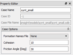
Case Constants
Two constants can be assigned to a Geomechanical case:
- Cohesion
- Friction angle
In the following they are denoted s0 and fa respectively. Some of the derived results use these constants, that can be changed in the property panel of the Case.
COMPACTION
Compaction is the difference in vertical displacement (U3) between a grid node and a specified reference K layer. The reference K layer is specified in the property editor.
For each node n in the grid, a node nref in the reference K layer is found by vertical intersection from the node n.
If Depthn <= Depthnref:
COMPACTIONn = -(U3n - U3nref)
else:
COMPACTIONn = -(U3nref - U3n)
ST - Total Stress
STii = -Saii + POR (i= 1,2,3)
STij = -Saij (i,j = 1,2,3 and i not equal j)
We use a value of POR=0.0 where it is not defined.
STi = Principal value i of ST
STM - Total Mean Stress
STM = (ST11 + ST22 + ST33)/3
Q - Deviatoric Stress
Q = sqrt( (3/2) * ( (ST1 – STM)2 + (ST2 – STM)2 + (ST3 – STM)2 ))
Gamma - Stress Path
Gammaii = STii/POR (i= 1,2,3)
Gammai = STi/POR
In these calculations we set Gamma to undefined if abs(POR) > 0.01 MPa.
SE - Effective Stress
SEij = -Saij (Where POR is defined)
SEij = undefined (Were POR is not defined)
SEi = Principal value i of SE
SEM - Effective Mean Stress
SEM = (SE11 + SE22 + SE33)/3
SFI
SFI = ( (s0/tan(fa) + 0.5(SE1 + SE3))sin(fa) ) /(0.5*(SE1-SE3) )
DSM
DSM = tan(rho)/tan(fa)
where
rho = 2 * (arctan (sqrt (( SE1 + a)/(SE3 + a)) ) – pi/4)
a = s0/tan(fa)
FOS
FOS = 1/DSM
E - Strain
Eij = -Eaij
EV - Volumetric Strain
EV = E11 + E22 + E33
ED - Deviatoric Strain
ED = 2*(E1-E3)/3
Element Nodal On Face
For each face displayed, (might be an element face or an intersection/intersection box face), a coordinate system is established such that:
- Ez is normal to the face, named N - Normal
- Ex is horizontal and in the plane of the face, named H - Horizontal
- Ey is in the plane pointing upwards, named QV - Quasi Vertical
The stress tensors in that particular face are then transformed to that coordinate system. The following quantities are derived from the transformed tensor named TS in the following:
SN - Stress component Normal to face
SN = TS33
TPH - Horizontal in-plane shear component
TPH = TS31 = TSZX
TNQV - Horizontal in-plane shear component
TPQV = TS32 = TSZY
TP - Total in-plane shear
TP = sqrt(TPH2 + TPQV2)
TPinc - Direction of TP
Angle of the total in-plane shear relative to the Quasi Vertical direction
TPinc = acos(TPQV/TP)
Pinc and Pazi - Face Inclination and Azimuth
These are the directional angles of the face-normal itself.